Wiener and Kolmogorov: The Birth of Modern Forecasting

Today we forecast markets, weather, or the spread of a virus using sophisticated mathematical models. But it all began in the midst of World War II, when two scientists — Norbert Wiener in the United States and Andrey Kolmogorov in the Soviet Union — tackled the same fundamental problem: how to predict the future from uncertain data.
Their solutions gave rise to the foundations of modern forecasting theory.

During World War II, Norbert Wiener (1894–1964), already a renowned mathematician and professor at MIT, was given a crucial task: to find a way to predict the trajectory of an enemy aircraft based on noisy and incomplete radar data.
The Allies could no longer afford to "guess" movements — they needed a system capable of accurately anticipating the target's behavior in real time, even in the presence of imperfect measurements and structural uncertainty.
Wiener met this challenge with an approach rooted in probabilistic analysis and frequency-domain transformations. The result was the now-famous Wiener Filter — a mathematical method for estimating the present or future value of a stationary signal, based on past observations, while minimizing the mean squared error (MSE).

In simple terms, Wiener showed how to optimally weigh past data to obtain the best possible prediction, even when the signal is buried in noise.
His work was initially compiled in a classified 1942 report titled Extrapolation, Interpolation, and Smoothing of Stationary Time Series (with Engineering Applications). Declassified only in 1949, the document had a tremendous impact across fields as diverse as electrical engineering, control systems, economics, and statistics.
Wiener’s contribution was not just theoretical — it was highly practical. He gave engineers a powerful tool for real-time forecasting and filtering, and laid the foundation for later techniques such as the Kalman Filter, which is still widely used today in navigation systems, robotics, finance, and advanced predictive models.

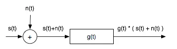
In reality, we cannot directly observe the clean signal. What we receive is a distorted version:

y(t) = s(t) + n(t) — that is, the sum of the true signal and noise.

This is where the Wiener filter comes into play, represented in the diagram as g(t). The filter is applied to the noisy signal y(t) to produce the best possible estimate of the original signal s(t), using only the information available.

The Wiener filter doesn’t treat all parts of the signal equally. Instead, it evaluates how strong the signal-to-noise ratio (SNR) is in each portion:

• If the signal is much stronger than the noise, the filter lets most of it pass through.

• If the noise is dominant, the filter suppresses or removes it.

The result is a cleaner version of the original signal — perhaps not perfect, but the best that can be achieved under the circumstances.

While Wiener was working on radar data and engineering applications, Andrey Kolmogorov (1903–1987) was quietly revolutionizing probability theory from within the Soviet Union.
In 1933, Kolmogorov had already achieved a groundbreaking milestone: he formalized probability as a rigorous branch of mathematics through his seminal work Foundations of the Theory of Probability. That work laid the axiomatic foundations that still guide the entire discipline today.
His next step was just as ambitious: to tackle the problem of forecasting from a general and abstract perspective, without tying it to any specific application. His key question was:

Given a stationary stochastic process — that is, a time series with stable mean and autocorrelation structure — what is the best possible linear predictor of its future values?

The answer came in the form of what we now call the Kolmogorov equations: a closed-form solution that allows us to compute the optimal forecast and its expected error, given the autocovariance function (or alternatively, the spectral density) of the process.
It was an extraordinary result: not only could the future be estimated with mathematical precision, but the uncertainty associated with the forecast could be quantified exactly.

Initially, this work remained little known in the West — due to both language barriers and the geopolitical tensions of the time — but as translations and interpretations began to spread, the theoretical depth of Kolmogorov’s contribution became increasingly clear.
His ideas became the theoretical foundation for a wide range of forecasting models, deeply influencing statistics, econometrics, and modern time series analysis.

Although Wiener and Kolmogorov approached the problem of forecasting from different perspectives — Wiener from the angle of real-time signal filtering, Kolmogorov from the abstract theory of probability — their insights converge on a fundamental principle:

The optimal linear forecastof a stationary time series can be derived from its second-order properties: the mean and the autocovariances.

This unified view became known as Wiener–Kolmogorov theory and represents the theoretical foundation of much of modern time series analysis.
Their work paved the way for models like the ARIMA family (AutoRegressive Integrated Moving Average), developed and popularized in the 1950s and still widely used today.

The contribution of Wiener and Kolmogorov transformed forecasting from an empirical intuition into a scientific method. It’s not just about calculating, but about understanding how much we can trust the result.
Their theory still provides the most robust answer to an eternal dual challenge: forecasting accuratelyandmeasuring uncertainty.

An ARIMA (AutoRegressive Integrated Moving Average) is a statistical model used for time series forecasting.
It is composed of three parts:

• AR (AutoRegressive): expresses the current value of the time series as a linear combination of its past values.

• I (Integrated): the series is differenced to make it stationary (i.e., constant mean and variance over time — a necessary condition for applying the model).

• MA (Moving Average): also accounts for past forecasting errors of the model.

An ARIMA model thus combines memory of historical values and past errors, applied to a stationary series, to generate future forecasts.
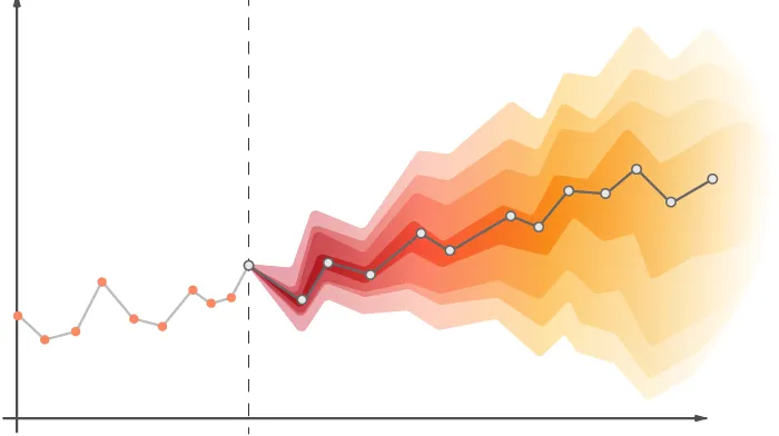
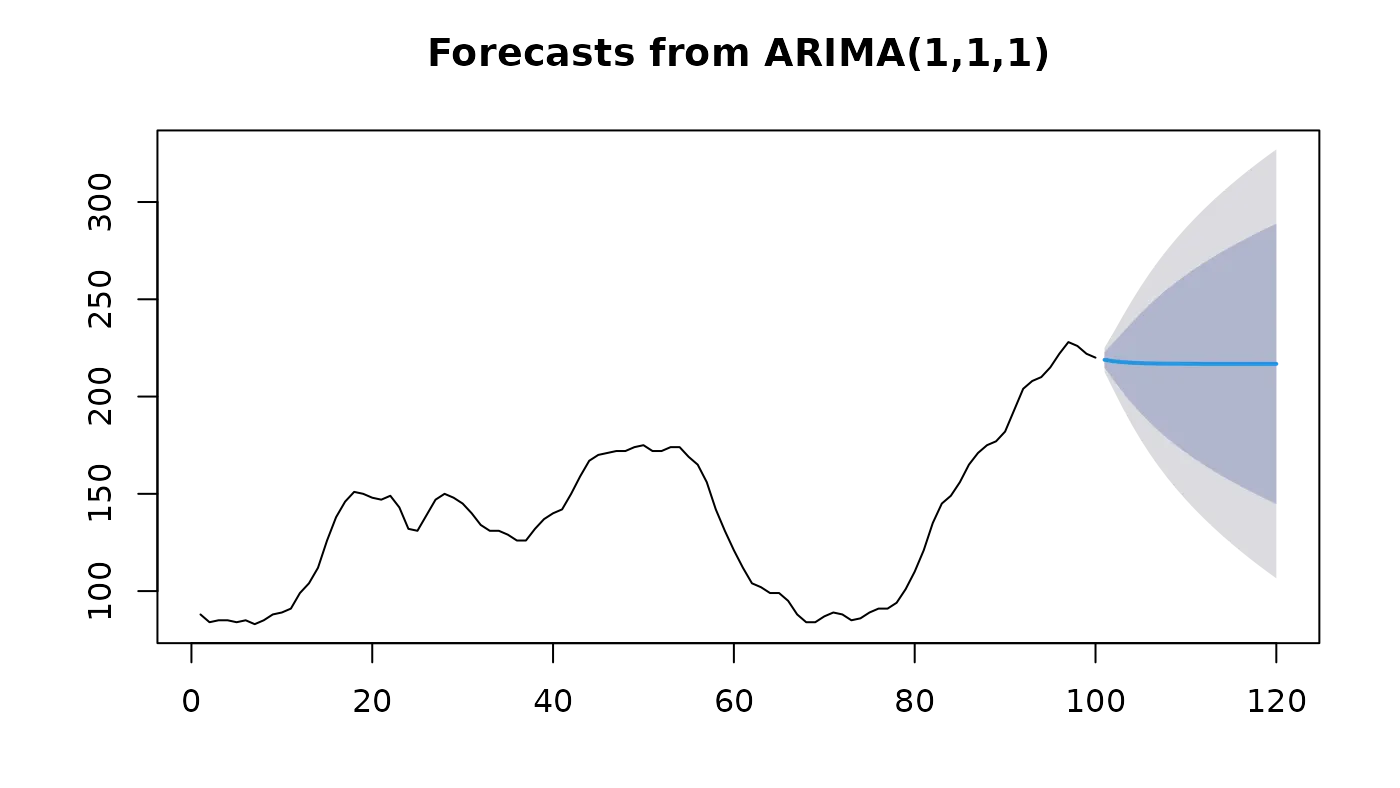
When forecasting with ARIMA (or other models), we don’t just get a prediction curve, but also a range of plausible future values.
This range is called a confidence interval and reflects the uncertainty of the forecast:

• The central line (blue in the image) is the point forecast.

• The gray/blue bands are confidence intervals (e.g., at 95%), indicating where future values are expected to fall with a certain probability.

The further into the future we forecast, the wider these intervals become → the model’s uncertainty increases.

We can’t predict everything — but we can learn to do it better and better. Thanks to Wiener and Kolmogorov, forecasting stopped being an approximate art and became a science grounded in logic, data, and uncertainty measurement.
And even today, every time we build a model or test a forecast, we’re walking the path they traced more than eighty years ago.

At Dhiria, we develop advanced predictive systems like TIMEX, designed to turn time series data into strategic decisions. By combining mathematical rigor, machine learning, and privacy-by-design, we deliver solutions ready to face real-world complexity.

👉 Discover how TIMEX can power your forecasting.
Visit www.dhiria.com